
GAWP - Generative art with Python
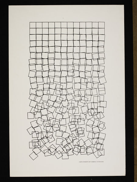
In 1965, programmer George Nees wrote his first pioneering works of generative art in ALGOL, printing his programs on punch cards and loading them into a Zuse Graphomat to plot them as physical drawings, including his well known Shotter.
The modern programmer has access to a vastly more convenient and powerful toolset, writing in a modern language, and drawing from the expansive ecosystem of open-source libraries available online.
Our tools
In this series of posts, I’ll be using Python to write programs that can generative svg images.
Python provides a great workspace for iterative creative work:
- It is a consise language with simple syntax in which you can achieve a lot with relatively little code
- It has a great ecosystem of open-source packages which can save you from reinventing the wheel by solving a problem that already has a good solution (for example, using a package that can generate SVG files, like svgwrite)
- As a scripting language you don’t have to worry about compiling your code as you make iterative changes to your program in order to tweak your work, accelerating your working process
SVG files provides a great file format for our generated images, for a few reasons:
- It’s a human-readable format (based on XML), so it’s easy to examine the output of your work and make manual changes
- It’s widely supported on browsers, making it easy to share your work
- It has all the advantages of vector images: it can be scaled without losing resolution and it can be used to generate physical drawings with a plotter
Getting started
A good practice for your Python projects is setting up a virtual environment for your packages. This will provide a self-contained environment where you can install specific versions of your packages in order to manage their dependencies and ensure intercompatibility between them, rather than using an operating system-level version of each package. There are many well known packages related to this subject (e.g. pipenv, virtualenv, venv, pyenv).
I’ve gone for virtualenv here. If you haven’t got it installed, run pip install virtualenv. Then, in your project folder, run virtualenv venv. This will create a directory called ‘venv’ which will contain installed packages.
We’ll be using the svgwrite package; running pip install svgwrite will install the package in that ‘venv’ directory, then we’ll create a .py file in which to write our code.
Examining a piece of generative art
Let’s take a look again at Shotter.
It’s essentially a grid of squares where their position and rotation becomes gradually more chaotic as their distance from the origin increases.
This should be simple to achieve with little more than a two-dimensional for loop and some random number generation.
In order to add progressive ‘chaos’, each square will have it’s own ‘origin’ position, modified by a random number whose possible range is larger for squares further from the origin. The same can be applied to its rotation.
Creating our own Shotter
First, let’s create a grid using svgwrite.
We can start by importing svgwrite and creating a single square of size 10 * 10 at co-ordinate (0,0) in the svg, and applying some global settings to the entire drawing. This handles most of our boilerplate.
import svgwrite

# Initialise the drawing
dwg = svgwrite.Drawing(
  'test.svg',
  size=(100, 100),
  profile='tiny',
  stroke_width=0.5,
  stroke='black',
  stroke_opacity=1.0
)

# Add the square
dwg.add(dwg.rect(
  (0, 0),
  (10, 10)
))

dwg.saveas("shotterOneSquare.svg")
Creating a grid of squares can be achieved with two nested for loops, running from 0 to 9. Their positions can be derived from the values ‘x’ and ‘y’, which increase by one with each loop. Bear in mind that higher ‘y’ values here will move the square further down the image, rather than up, because the origin (0, 0) is in the top left hand corner of the image.
import svgwrite

dwg = svgwrite.Drawing(
  'test.svg',
  size=(100, 100),
  profile='tiny',
  stroke_width=0.5,
  stroke='black',
  stroke_opacity=1.0,
  fill='none'
)

width = 10
height = 10

for x in range(0, width):
    for y in range(0, height):
        dwg.add(dwg.rect(
        (x * 10,y * 10),
        (10,10)
        ))

dwg.saveas("shotterGrid.svg")
Adding chaos
We now have a plain 10 * 10 grid of squares. Python’s random package from the standard library can help us introduce some chaos.
First, we import random, then we:
- Create x and y position modifiers for each square during our loop using
random.random()(which generates a pseudo-random floating point number between 0.0 and 1.0) - Minus 0.5 from the randomly generated number, so that we have a number between -0.5 and 0.5
- Multiply this modifier by the ‘number’ of the current square, for example 1 for the first square in the first row, 11 for the first square in the second row (given by
x + (y * width)) so that squares further from the origin can be moved a greater distance.
import svgwrite
import random

dwg = svgwrite.Drawing(
  'test.svg',
  size=(100, 100),
  profile='tiny',
  stroke_width=0.5,
  stroke='black',
  stroke_opacity=1.0,
  fill='none'
)

width = 10
height = 10

for x in range(0, width):
    for y in range(0, height):
        position_modifier_x = (random.random() - 0.5) * (x + (y * width))
        position_modifier_y = (random.random() - 0.5) * (x + (y * width))
        dwg.add(dwg.rect(
            (
                x * 10 + position_modifier_x,
                y * 10 + position_modifier_y
            ),
            (10,10)
        ))

dwg.saveas("shotterGridPosition.svg")
The result is overly chaotic, but with some minor numerical tweaking, we can achieve something more similar to Nees’ Shotter.
import svgwrite
import random

dwg = svgwrite.Drawing(
  'test.svg',
  size=(100, 100),
  profile='tiny',
  stroke_width=0.5,
  stroke='black',
  stroke_opacity=1.0,
  fill='none'
)

width = 10
height = 10
dampener = 100

for x in range(0, width):
    for y in range(0, height):
        position_modifier_x = (random.random() - 0.5) * (x + (y * width)) * y / dampener
        position_modifier_y = (random.random() - 0.5) * (x + (y * width)) * y / dampener
        dwg.add(dwg.rect(
            (
                x * 10 + position_modifier_x,
                y * 10 + position_modifier_y
            ),
            (10,10)
        ))

dwg.saveas("shotterGridPositionTweaked.svg")
In order to add rotation to the squares, we can add a rotate transformation to each square. We will subtitute the rotation degree and centre co-ordinate values into a transformation using an f-string along the following lines: transform=f"rotate({degrees}, {centre_x_coord}, {centre_y_coord})"
import svgwrite
import random

dwg = svgwrite.Drawing(
  'test.svg',
  size=(100, 100),
  profile='tiny',
  stroke_width=0.5,
  stroke='black',
  stroke_opacity=1.0,
  fill='none'
)

width = 10
height = 10
position_dampener = 100
rotation_dampener = 10

for x in range(0, width):
    for y in range(0, height):
        position_modifier_x = (random.random() - 0.5) * (x + (y * width)) * y / position_dampener
        x_position = x * 10 + position_modifier_x

        position_modifier_y = (random.random() - 0.5) * (x + (y * width)) * y / position_dampener
        y_position = y * 10 + position_modifier_y

        rotation = (random.random() - 0.5) * (x + (y * width)) * y / rotation_dampener

        dwg.add(dwg.rect(
            (x_position,y_position
            ),
            (10,10),
            transform = f"rotate({rotation},{x_position + 5},{y_position +5})"
        ))

dwg.saveas("shotterGridPositionWithRotation.svg")
Which generates this:
Finishing up
We really have everything we need. A few minor changes to the program can create something very similar to what George Nees produced, and we can tidy our code using functions to reduce repetition (I’ve used lambda functions but standard functions would work just as well).
import svgwrite
import random

dwg = svgwrite.Drawing(
  'test.svg',
  size=(100, 100),
  profile='tiny',
  stroke_width=0.5,
  stroke='black',
  stroke_opacity=1.0,
  fill='none'
)

width = 10
height = 20
position_dampener = 400
rotation_dampener = 15

random_magnitude = lambda x,y : (random.random() - 0.5) * (x + (y * width)) * y
random_position_magnitude = lambda x,y : random_magnitude(x,y) / position_dampener

for x in range(0, width):
    for y in range(0, height):
        position_modifier_x = random_position_magnitude(x,y)
        x_position = x * 10 + position_modifier_x

        position_modifier_y = random_position_magnitude(x,y)
        y_position = y * 10 + position_modifier_y

        rotation = "{:.1f}".format(random_magnitude(x,y) / rotation_dampener)

        dwg.add(dwg.rect(
            (x_position,y_position
            ),
            (10,10),
            transform = f"rotate({rotation},{x_position + 5},{y_position + 5})"
        ))

dwg.saveas("shotter.svg")
It’s worth bearing in mind that we haven’t produce a single artwork here - what we have made is a program that can produce myriad artworks following the algorithm, or set of rules, that we have written.
Here are a set of images produced by our program: